Why Artesis Omnisight Is a Revolutionary Solution for Predictive Maintenance

Most condition monitoring programs are architected around a tiering decision that gets made once, early, and rarely revisited: a handful of motors above some horsepower or criticality threshold get permanent instrumentation, everything else gets a walk-around route if it gets anything at all, and the two data sets live in separate systems maintained by separate teams. The tiering decision isn’t wrong on its face — capital allocation has to stop somewhere — but the architecture it produces creates a specific and predictable failure mode: assets just below the cutoff degrade without anyone building a trend on them, because the tools used to watch the top tier and the tools used to spot-check everything else don’t share a data model, an alarm taxonomy, or in most cases a common analyst.

Artesis Omnisight

Artesis Omnisight addresses this by collapsing that architecture into a single electrical signature analysis (ESA) pipeline that serves both continuous and route-based deployments, and the technical reasoning behind that consolidation is worth unpacking in more detail than the marketing copy usually goes into.

Why Fragmented Monitoring Fails at the Signal Level, Not Just the Organizational Level

Vibration-based programs typically split by sensor type and mounting method: permanently wired accelerometers on critical assets, versus a technician walking a route with a handheld collector and magnet-mounted transducers on secondary equipment. These aren’t just two workflows — they’re two different measurement chains, with different sampling rates, different transducer frequency response characteristics, and often different FFT resolution and windowing parameters between the fixed system and the portable unit. A bearing defect frequency calculated against nameplate RPM on one system doesn’t always reconcile cleanly against the same calculation run through a different vendor’s portable analyzer, particularly once shaft speed varies under VFD control.

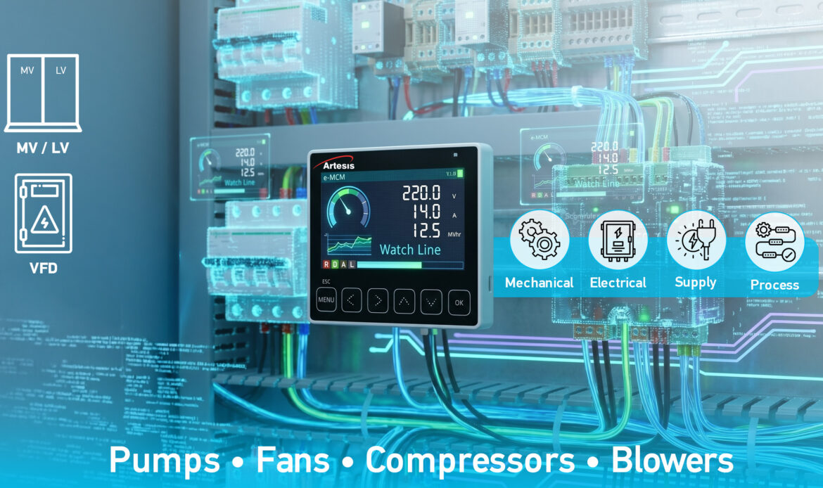
ESA sidesteps this specific problem because the measurement point is electrical rather than mechanical: current and voltage at the motor terminals or MCC, sampled and processed to extract sidebands around the line frequency and its harmonics. Mechanical fault frequencies — bearing defect frequencies (BPFO, BPFI, BSF, FTF), rotor bar pass frequency, eccentricity-related pole-pass sidebands — all modulate the stator current at frequencies that can be derived directly from slip and synchronous speed, independent of the physical sensor placement that trips up cross-platform vibration comparisons. Whether the current waveform is captured continuously from a permanently installed CT/PT set (eMCM) or during a scheduled walk-around using a portable clamp-on unit (AMTPro), the underlying spectral processing and fault-frequency derivation are the same. That’s the technical basis for putting both deployment modes into one dataset rather than two.

What Omnisight Actually Computes

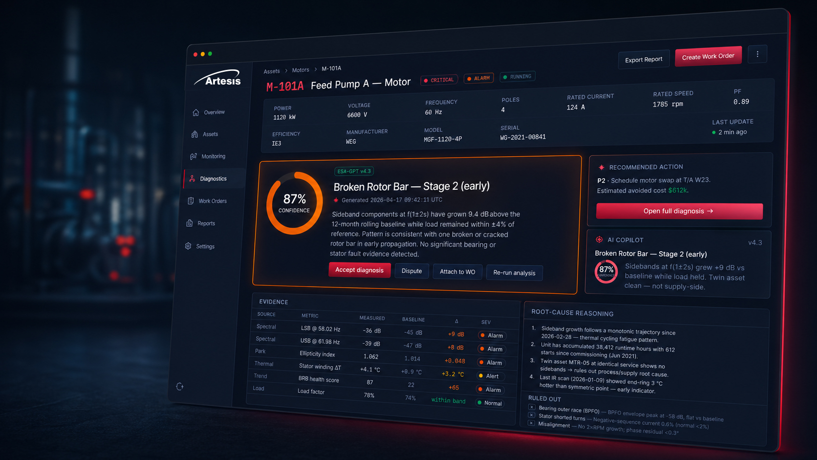
The processing chain runs roughly as follows: current and voltage waveforms are sampled at the motor or MCC, a high-resolution FFT is applied to extract the current spectrum around the fundamental and relevant harmonics, and sideband amplitudes at calculated fault frequencies are compared against baseline severity indices established during commissioning or early operation. For rolling-element bearings this means tracking sideband energy at BPFO/BPFI relative to the fundamental slot-passing components; for rotor bar and end-ring conditions it means monitoring the twice-slip-frequency sidebands around the fundamental; for eccentricity it’s the pole-pass frequency components superimposed on the supply harmonics. None of this requires a vibration sensor to be present at all — it’s derivable from the same current signal already available at any MCC breaker or starter, which is why the deployment cost profile for extending coverage past the critical-asset tier looks so different from adding another accelerometer and cable run.

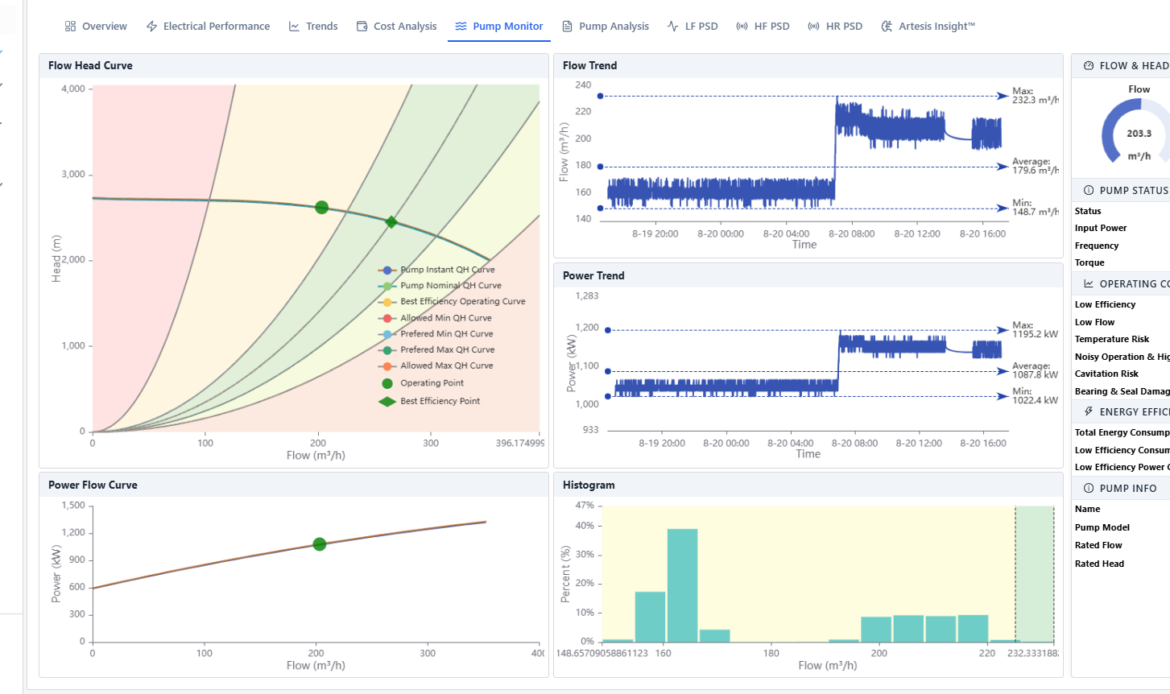
Severity indices get trended over time rather than evaluated against a fixed absolute threshold, because absolute sideband amplitude at a given fault frequency is itself a function of load — a motor running at 60% of rated torque produces different baseline sideband energy than the same motor at 95%, independent of mechanical condition. Omnisight’s baselining accounts for this by normalizing against load and speed at the time of each measurement rather than flagging deviation from a single static setpoint, which is the detail that keeps a load-dependent asset like a conveyor drive or a variable-duty pump from generating nuisance alarms every time production ramps up.

What is predictive maintenance?

Interpretation Layer: Artesis Insight

Raw sideband severity indices and trend slopes are not directly actionable for most maintenance technicians without training in motor current signature analysis, so Omnisight routes processed indicators through Artesis Insight, which maps the measured indices to a plain-language condition statement and an estimated remaining runway — for example, translating a specific BPFO sideband trend and its rate of change into an estimate along the lines of three to four months before inspection is warranted, rather than reporting a raw dB value against a fault frequency that only an ESA specialist would parse correctly. This matters operationally because it decouples “who captures the data” from “who needs formal training to interpret a current spectrum” — a technician running an AMTPro route doesn’t need MCSA certification to act on the output, since the interpretation step has already been done upstream.

Coverage Economics: Where the Marginal Cost Actually Changes

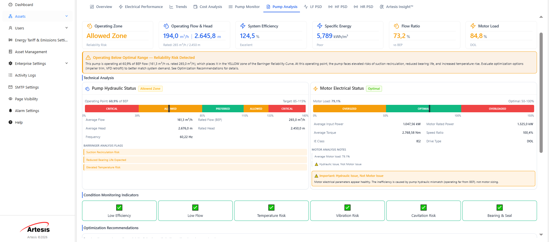
Extending a permanently wired eMCM installation to another asset means another CT/PT set, another data acquisition channel, and in many facilities, panel space and cabling work inside an already congested MCC. Extending AMTPro coverage to another asset means adding a measurement point to an existing walk-around route — no new hardware per asset, no panel modification, and no continuous data channel to provision. Because both feed the same severity-index model and the same Insight interpretation layer, a facility can run continuous ESA on its top 10-15 assets by criticality and consequence-of-failure, and extend the same fault-frequency methodology across the remaining fleet at route intervals — weekly, monthly, whatever cadence the asset’s risk profile justifies — without switching methodologies or reconciling two incompatible fault-frequency baselines.

The Practical Difference

The net effect is that assets historically excluded from any condition-based program purely on a cost basis — secondary pumps, auxiliary fans, non-critical conveyor drives — get evaluated with the same fault-frequency rigor as the assets already on continuous monitoring, at whatever measurement cadence the plant can justify economically. That’s a different proposition than most legacy monitoring architectures offer, where extending coverage below the critical tier has historically meant either a second, less rigorous methodology or no coverage at all.